Chapter 14
Reserves
Oil reserves classification: proved, probable, possible, reserve replacement ratios, Hubbert peak oil theory, and resource estimates.
An oil company executive was interviewing three potential employees, a geologist, a geophysicist, and a petroleum engineer (the kind that estimates reserves). One question asked was: "What is two times two?" The geologist answered that it was probably more than three and less than five, but the issue could use some more research. The geophysicist punched it into his computer and announced that it was 3.999999. The petroleum engineer jumped up and locked the door, closed the window blinds, unplugged the phone, and asked quietly, "What do you want it to be?"
Adapted from Deffeyes, K.S. (2005)
What Are Oil Reserves?
There are no universally accepted definitions of oil reserves. Industry groups, regulators, and governments each maintain their own frameworks. The total crude oil in a region, both discovered and undiscovered, is called Original Oil In Place (OOIP). Resources are the portion estimated to be technically feasible to recover. Reserves are the subset of resources estimated to be both technically and economically producible at prevailing prices and with current technology. A fourth concept, Estimated Ultimate Recovery (EUR), is the cumulative volume a well or field is expected to produce over its entire life, from first flow to abandonment. EUR is the number that matters most to an engineer planning a drilling program, while reserves are the number that matters most to a banker sizing a loan.
Reserves sit at the intersection of geology, technology, price, and contract law. A 2005 barrel uneconomic at $30 crude became a reserve at $80 crude, then quietly dropped off the books again when the price fell below $40 in 2015. No physical barrels moved. The SEC's 12-month trailing average price test, Canada's NI 51-101, the Society of Petroleum Engineers' PRMS, and Russia's own state reserve classification all produce different numbers for the same underground pool. Treat any single reserve figure as an opinion with a methodology attached, not a fact.
The Three Ps
Reserves are classified by probability. Proven (P1 or P90) reserves have at least a 90% probability of being produced under current economic and technical conditions. Probable (P2 or P50) reserves have a best-estimate probability of about 50%. Possible (P3 or P10) reserves have roughly a 10% probability of being recovered. The labels P90, P50, and P10 come from the cumulative probability distribution used by petroleum engineers: P90 means there is a 90% chance the true recoverable volume is at least as large as the stated number. Adding proven plus probable gives 2P reserves; adding proven plus probable plus possible gives 3P. Industry operators and private lenders often work from 2P; only 1P (proven) can be counted as assets under US GAAP for SEC filings.
The SEC updated its oil and gas reporting rules in late 2008, effective for 2009 annual reports. The new rules permit 3-D seismic and other reliable technology to establish reserves without a drill bit in the ground, recognize oil sands and bitumen as oil reserves rather than mining assets, and replace the old single-day year-end price with a 12-month trailing average of first-of-month prices. That last change was a direct response to the whipsaw of 2008, when a $147 July WTI print and a $33 December print would have produced wildly different book reserves under the old rule.
PDP, PDNP, PUD: The Development Status Categories
Within proven reserves, US SEC reporting requires a further breakdown by development status. PDP (Proved Developed Producing) reserves are barrels expected to be recovered from wells already drilled, completed, and currently flowing. PDNP (Proved Developed Non-Producing) covers wells that are drilled and completed but temporarily shut in, behind-pipe zones awaiting recompletion, or wells waiting on a pipeline tie-in. PUD (Proved Undeveloped) reserves are barrels assigned to locations that have not yet been drilled but are scheduled for development within five years of being booked.
Table 14-1: Proved Reserve Development Categories
| Category | Status | Capital Required |
|---|---|---|
| PDP | Drilled, completed, and currently producing | None (operating costs only) |
| PDNP | Drilled and completed but not flowing (shut-in, behind-pipe, awaiting tie-in) | Minor (workover or hookup) |
| PUD | Undrilled locations scheduled for development within 5 years | Full drilling and completion cost |
Reserve Recategorization ("Re-Catting")
Because the three categories carry very different capital requirements and risk profiles, reserve auditors and lenders watch closely for movement between them. Shifting a barrel from PUD to PDP through successful drilling is the normal value creation cycle for an E&P company. The reverse, however, is a warning sign. Recategorization, known in the industry as "re-catting", is the reclassification of barrels from a higher-confidence category to a lower one, or out of proved reserves entirely.
Re-catting typically happens for three reasons. First, the SEC five-year rule: any PUD location that will not be drilled within five years of its initial booking must be removed from proved reserves, even if the geology has not changed. Second, a sustained drop in commodity prices can make previously economic barrels uneconomic at the SEC 12-month average price test, forcing negative price revisions. Third, drilling results from offset wells can show that the original geological assumptions were too optimistic, triggering performance revisions.
Negative revisions are scrutinized by reserve-based lenders (RBLs) because the borrowing base of an E&P credit facility is sized off PDP reserves at lender price decks. A material PUD-to-unproved write-down can also force an accounting impairment, though which test applies depends on the accounting method the company elected. Under full cost accounting, every exploration cost, including dry holes, is capitalized into a single country-wide pool, and SEC Regulation S-X Rule 4-10 caps the book value of that pool at a ceiling, defined as the after-tax PV-10 of proved reserves calculated at the same 12-month trailing average price used to book the reserves themselves. If carrying value exceeds that ceiling, the excess is written off at once, and the write-off cannot be reversed if prices later recover. Under successful efforts accounting, dry holes are expensed as they are drilled rather than capitalized, and there is no SEC ceiling test at all. Impairment is assessed field by field under ASC 360, against the company's own price forecast rather than the SEC average.
The practical difference is timing and sensitivity. Because the full cost ceiling is recalculated every quarter off a trailing average price the company does not choose, full cost filers took large and well-publicized ceiling test write-downs in 2015 and again in 2020, while successful efforts filers holding comparable rock often reported none. Two companies can own the same barrels and report very different book values for them, which is one more reason to read a reserve disclosure alongside the accounting policy note rather than on its own.
For analysts, the year-over-year change in reserves should always be decomposed into four buckets: extensions and discoveries, improved recovery, purchases or sales, and revisions. The revisions line is where re-catting shows up, and it separates further into two kinds that carry opposite signals.
A technical revision reflects new information about the rock: an offset well that produced above or below its type curve, a reprocessed seismic volume, or an updated decline-curve fit. Technical revisions divide again into performance revisions, where existing wells beat or miss the original forecast, and recategorizations, where volumes previously carried as probable or possible are promoted into proved without a single new well being drilled. An economic revision reflects no new information about the rock at all. A change in price, operating cost, or fiscal terms moves the economic limit of existing wells, meaning the point at which revenue stops covering the cost of lifting the next barrel, and barrels cross into or out of proved on that basis alone. The distinction governs how a reader should treat the number. An economic revision reverses when the price does. A negative technical revision means the reservoir is genuinely smaller than the company believed, and those barrels do not come back.
Reserve Estimation Methods
Reservoir engineers have four main quantitative tools for estimating how much oil a field will produce, plus a fifth rule-of-thumb analogy method used before any real data is in hand. The appropriate tool depends on how much of the field's life has already elapsed, what data is available, and how mature the surrounding basin is. Different methods are often run in parallel and cross-checked.
The volumetric method is the earliest-life approach. Before any material flow from the reservoir, engineers combine seismic, well log, and core data to estimate pay zone area, net pay thickness, porosity, hydrocarbon saturation, and a formation volume factor, then back out a volume. It is the only option for a discovery that has been drilled and logged but not produced, and it feeds the OOIP number that every recovery factor is later applied to.
Material balance kicks in once the reservoir has produced enough fluid for its pressure to fall measurably. The technique treats the reservoir as a closed tank: the drop in pressure for each barrel produced tells the engineer how much oil, gas, and water were originally in place, assuming reasonable values for rock and fluid compressibility and aquifer support. Material balance is powerful because it relies on actual production data rather than log estimates, but it requires a coherent pressure history and is difficult in tight rock where pressure communication is poor.
Decline curve analysis is the workhorse of mature fields. Once a well is past its peak, its rate typically falls along a predictable curve, exponential, hyperbolic, or harmonic, described by an initial rate, an initial decline rate, and a hyperbolic exponent. Fitting that curve to the first one to three years of production and extrapolating forward gives an EUR for each well, which is then summed up to field level. Decline curves are heavily used in shale, where the very steep first-year decline and flat tail make forecasting sensitive to the chosen exponent and economic cutoff.
Figure 14-1: Arps Decline Curves
Reservoir simulation is the most data-hungry method. A 3-D grid of the reservoir is built from seismic and well data, populated with rock and fluid properties, and then flowed numerically through time, with each grid cell exchanging fluids with its neighbors according to Darcy's law and local pressure gradients. A well-tuned simulation can answer questions no other method can: what happens if we infill drill here, if we inject CO2 there, if we convert this producer to a water injector. It is also slow, expensive, and only as good as the history match that calibrates it to actual production.
Worked example: the volumetric method. The standard field formula for original oil in place, in US oilfield units, is:
OOIP (bbl) = (7758 × A × h × φ × (1 - Sw)) / Bo
where A is drainage area in acres, his net pay thickness in feet, φ is porosity as a fraction, Sw is connate water saturation as a fraction, and Bo is the oil formation volume factor (reservoir barrels per stock-tank barrel). The 7758 is the number of barrels in one acre-foot. For a modest example, take A = 1,000 acres, h= 50 ft, φ = 0.20, Sw = 0.25, and Bo = 1.2. Then:
OOIP = (7758 × 1000 × 50 × 0.20 × 0.75) / 1.2 ≈ 48.5 million bbl
That is oil in place, not reserves. Apply a recovery factor, roughly 30% for a primary-and-waterflood conventional field or 7% to 10% for unstimulated shale, and you arrive at recoverable reserves. The arithmetic is simple. The argument is always about the inputs.
Table 14-2: Reserve Estimation Methods
| Method | Description | Phase |
|---|---|---|
| Nominal | Rule-of-thumb analogy to known fields | Pre-production |
| Volumetric | Geological data on porosity, saturation, pay thickness | Pre-production |
| Material Balance | Reservoir pressure measurements over time | Early production |
| Decline Curve | Extrapolation of production decline rates | Declining production |
| Reservoir Simulation | Complex computer models using multiple data sources | Any stage |
Peak Oil and Hubbert's Curve
In 1956, Shell geophysicist M. King Hubbert presented a paper to the American Petroleum Institute that would become one of the most famous forecasts in petroleum history. His subject was the Lower 48, the industry's standing shorthand for the 48 contiguous US states, excluding Alaska and Hawaii. That exclusion is substantive rather than clerical. Alaska was not yet a state when Hubbert wrote, Prudhoe Bay would not be found for another twelve years, and when Alaskan crude finally arrived in 1977 it produced a second and entirely separate production pulse that would have obscured the decline he was describing. The Lower 48 is the geography in which the peak-oil argument was originally made, and it is still the series analysts reach for when they want US production with the Alaskan step-change taken out.
Hubbert observed that Lower 48 discoveries had peaked in the 1930s and argued that production would follow roughly 35 years behind, tracing a symmetric bell-shaped logistic curve that rose as the easy barrels were found and fell as the industry worked through progressively harder rock. He drew two cases rather than one. His most likely case assumed 150 billion barrels of ultimate recovery and peaked in 1965 at about 7.7 Mbpd. His upper-bound case assumed 200 billion barrels and peaked in 1970 at about 8.2 Mbpd. Lower 48 crude output in the event topped out at 9.8 Mbpd in November 1970, then began a long decline that continued until 2008. Hubbert had the year right in his upper-bound case and the rate roughly 15 percent too low, which remains a better result than anything the forecasters who dismissed him produced.
Shell's head office learned what was in the paper before Hubbert delivered it and spent the days beforehand trying to get the peak prediction taken out. One executive asked him, in Hubbert's recollection, "Couldn't you tone it down a bit? Couldn't you take the sensational parts out?" The calls from Houston continued until roughly five minutes before he stood up to speak in San Antonio on the morning of March 8, 1956. He delivered the paper as written. The most famous forecast in the history of the oil industry was made by an employee ignoring his own company's instructions not to make it.
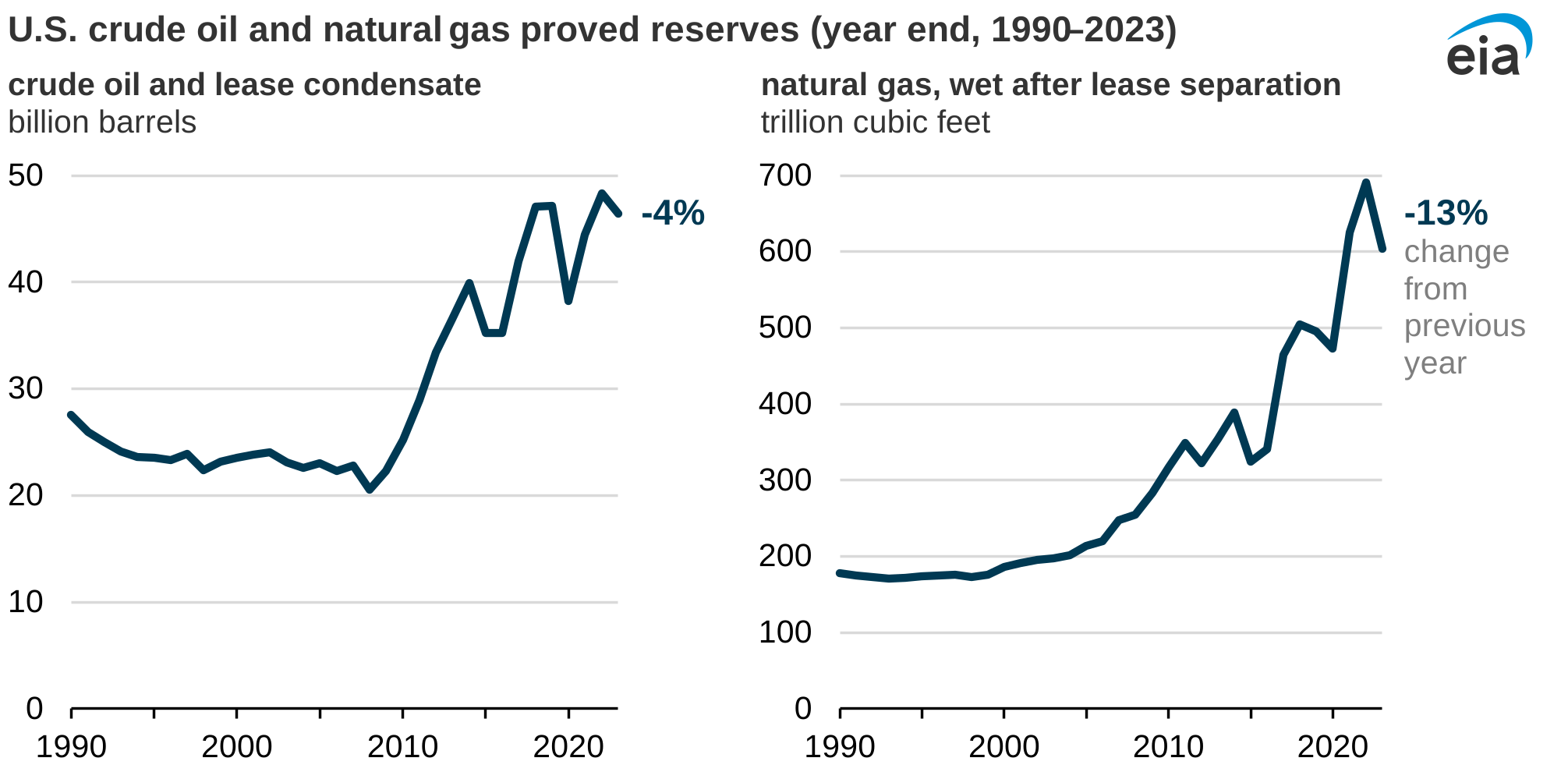
Hubbert was right about the physics and wrong about the economics. His model assumed a fixed resource base, but the resource base is a function of price and technology. Horizontal drilling and hydraulic fracturing turned source rocks, which Hubbert had classified as non-reservoir, into the most productive oil plays in the world. US crude production crossed back through its 1970 peak in 2018 and reached roughly 13.5 Mbpd by 2025. The Hubbert curve remains a useful mental model for a single conventional field where geology imposes a bell shape, but not for a country whose industry can redefine "reservoir" every twenty years.
Figure 14-3: Hubbert 1956 Prediction vs Actual US Lower-48 Crude Oil Production
OPEC's 1982-1988 Reserve Revisions
Any discussion of global reserves has to grapple with what happened inside OPEC between 1982 and 1988. The cartel's quota system linked each member's allowed output to its stated reserves. Larger reserves meant a larger quota, meant larger revenue. Over those six years, six OPEC members added more than 300 billion barrels to their stated proved reserves without corresponding discoveries. Some revisions doubled or tripled reported figures in a single year. No major new fields were announced. No new drilling campaigns justified the revisions. The numbers simply moved.
Table 14-3: OPEC Reserve Additions, 1982-1988 (no major new discoveries)
| Country | Increase | Context |
|---|---|---|
| Kuwait | +41% | Revision booked 1985 |
| Venezuela | +77% | Extra-heavy Orinoco belt reclassified |
| Iran | +91% | Post-war catch-up to Iraq |
| Iraq | +103% | Doubled in 1987 mid Iran-Iraq war |
| Saudi Arabia | +51% | 1988 revision, no field-level detail |
| UAE | +198% | Largest proportional increase |
These same countries have since produced hundreds of billions of barrels without materially writing their reserves down, which is arithmetically difficult to reconcile with any orthodox reserve-accounting framework. Saudi Aramco's 2019 bond prospectus, the first independent audit of Saudi reserves in decades, broadly confirmed the Saudi figure, but the other revisions remain unaudited. The practical takeaway is that the trillion-barrel-plus figure for OPEC proved reserves carries a large political component that does not exist in SEC-filed private-sector numbers.
Reserves to Production Ratio by Country
The Reserves to Production ratio (R/P) is the simplest possible durability metric: stated proved reserves divided by current annual production, expressed in years. It is a snapshot answering one narrow question, namely how many years the current booked pile would last at today's flow rate. It forecasts neither how long oil will last nor the expected producing life of any individual field. The ratio moves constantly as production changes and as reserves are revised, and it carries forward all the political baggage of the stated reserves in the numerator.
Table 14-4: R/P Ratio by Country (approximate, year-end 2024)
| Country | Proved reserves (bn bbl) | Production (Mbpd) | R/P (years) |
|---|---|---|---|
| Venezuela | 303 | 0.7 | >300 |
| Saudi Arabia | 267 | 11.1 | 65 |
| Iran | 209 | 3.8 | 140 |
| Canada | 167 | 5.7 | 80 |
| Iraq | 145 | 4.2 | 90 |
| UAE | 113 | 3.8 | 80 |
| Kuwait | 102 | 2.9 | 95 |
| Russia | 80 | 10.7 | 20 |
| United States | 74 | 13.4 | 15 |
| Libya | 48 | 1.2 | 110 |
| China | 26 | 4.1 | 17 |
| Global total | 1,700 | 96 | 50 |
Venezuela's 303 billion barrels, most of it Orinoco extra-heavy oil requiring upgrading and dilution, carries a very different recovery cost and quality than Saudi Arabian Light crude. The R/P ratios for OPEC members are all inflated by the 1980s revisions. The US and Russia sit at the other extreme: highly active production bases with relatively short booked life, because private operators book reserves conservatively and because SEC five-year PUD rules cap how far into the future a shale operator can reach. A short US R/P is not a supply warning, it is a feature of the accounting regime.
Figure 14-4 Top 15 Countries by Proved Oil Reserves (Billion Barrels)
Source: BP/Energy Institute Statistical Review 2024, OPEC Annual Statistical Bulletin. OPEC members hold roughly 70% of global proved reserves.
Reserve Replacement Ratio
For a publicly traded E&P company, the critical annual question is whether new reserves were added faster than old reserves were produced. The Reserve Replacement Ratio (RRR) measures this directly:
RRR = (reserves added through extensions, discoveries, revisions, and acquisitions) / production
Two details decide whether a given RRR figure means anything. The first is which reserve category is being counted. For SEC filers the ratio is calculated on proved (1P) reserves, because proved is the only category the SEC permits in a 10-K, so numerator and denominator are both SEC-basis barrels priced off the 12-month trailing average. Companies reporting under Canada's NI 51-101 or the SPE's PRMS may quote a 2P-based ratio instead, which is a different and generally more flattering number, so the headline percentages are not comparable across reporting regimes. The second is whether acquisitions are counted. The formula above is the total RRR. Strip out purchases and sales and what remains is the organic RRR, the barrels the drill bit and the geologists actually delivered. A company can post a total RRR of 150 percent by writing a cheque, which is why analysts quote the organic figure and treat a large gap between the two as the more informative number.
An RRR above 100% means the company is growing its reserve base; sustained readings below 100% mean it is liquidating. The table below shows recent reported RRRs for a handful of majors. The post-pandemic trend has been worrying: with capex cut sharply in 2020 and only a partial rebound since, the IOC peer group average has dipped below 100%, meaning the majors as a group are not replacing what they pump. ExxonMobil and ConocoPhillips, the two most US-shale-weighted names, are the clear positive outliers.
Table 14-5: Reserve Replacement Ratios, Recent Annual (approximate)
| Company | Recent RRR | Note |
|---|---|---|
| ConocoPhillips | 140% | Permian + Alaska extensions |
| ExxonMobil | 120% | Guyana + Permian |
| TotalEnergies | 100% | LNG and deepwater |
| Chevron | 98% | Permian growth offset by divestitures |
| Shell | 78% | Active portfolio high-grading |
| BP | 67% | Post-strategy-reset, deliberate shrink |
SEC PV-10 and Reserve-Based Lending
Proved reserves are not just a production forecast, they are the collateral that backs a large fraction of independent E&P debt. PV-10 (present value at a 10% discount rate) is the discounted pre-tax cash flow from a company's proved reserves, calculated under the same SEC 12-month trailing average price rule that governs reserve volumes. Every 10-K filed by a US oil and gas producer includes a PV-10 figure, and every reserve-based lending (RBL) facility uses an internal version of it to size the borrowing base.
RBL lenders do not simply accept the company's PV-10. They re-run the cash flow under their own, usually more conservative, price deck, typically called the "bank price deck," apply their own advance rates to PDP, PDNP, and PUD categories (PDP gets the highest advance rate, PUD the lowest), and recalculate the borrowing base twice a year in spring and fall redeterminations. A sharp price drop between redeterminations, or a reserve recategorization that moves barrels out of PDP, can trigger a borrowing base cut that forces asset sales or equity issuance. This is why re-catting is a credit event, not merely an accounting footnote.
EUR and Drilling Inventory
In the shale era, the key operational number is Estimated Ultimate Recovery per well and the count of remaining Tier 1 locations in the company's inventory, rather than booked reserves. Tier 1 inventory is the number of undrilled locations a company holds in the best rock it controls, the part of a play where thickness, porosity, pressure, and oil saturation combine to deliver the highest return per well at a given price. No regulator defines the term, no reserve auditor certifies it, and each operator sets its own threshold, so one company's Tier 1 is another's Tier 2. The boundary also has a habit of moving outward as the best rock is consumed and a company needs to show that it still has runway.
Analysts talk about "decades of Tier 1 inventory" as a marketing claim and regulators largely let it stand, because the SEC five-year PUD rule prevents most of that inventory from ever being booked as reserves. The result is a two-tier disclosure regime: booked reserves for the SEC, inventory counts for the earnings call. Both matter, and they do not always tell the same story. Chapter 21 (Shale Revolution) returns to this tension and its finite Tier 1 runway.
Giant Fields Still Dominate Global Reserves
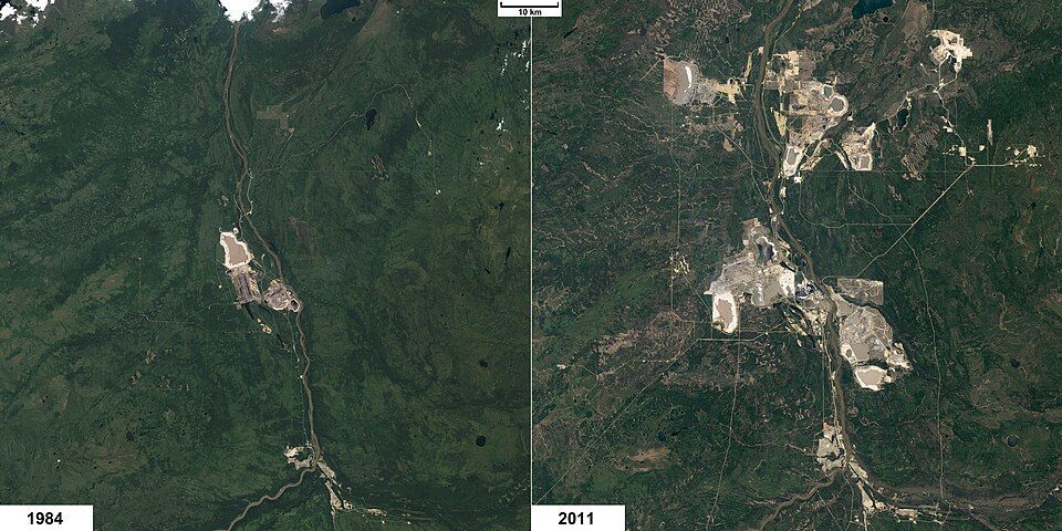
Despite the shale revolution, conventional giant fields (recoverable reserves of 500 million barrels of oil equivalent or more) still hold the majority of global proven reserves. A 2014 study by Guoping Bai and Yan Xu at the China University of Petroleum, published in the Oil and Gas Journal, documented that since 2000 the industry discovered 52 giant oil fields and 68 giant gas fields with combined 2P reserves of 248.6 billion barrels of oil equivalent. These fields cluster in seven regions.
Table 14-6: Giant Fields Discovered Since 2000 by Region
| Region | Giant fields |
|---|---|
| Middle East | 28 |
| Offshore Brazil | 19 |
| Offshore East Africa | 13 |
| Central Asia | 9 |
| NW Australia | 8 |
| Offshore West Africa | 6 |
| Gulf of Mexico | 5 |
Table 14-7: Top Basins by Share of Giant Field 2P Reserves (2000-2012)
| Basin | Share of total |
|---|---|
| Amu-Darya | 27.0% |
| Santos | 13.2% |
| Arabian | 9.8% |
| North Caspian | 7.6% |
| Zagros | 6.9% |
| Tanzania | 6.8% |
Marine carbonate reservoirs host 54.5 percent of the total giant field reserves discovered since 2000, followed by turbidites (17.6 percent), clastics (15.9 percent), and lacustrine carbonates (12.0 percent). Those four labels describe the rock the oil is sitting in, and each one is a different story about how that rock came to be there.
- Marine carbonates are limestones and dolomites built from the shells, skeletons, and reefs of shallow tropical seas. This is the rock that holds Ghawar and most of the Middle East, which is why one category alone accounts for more than half the table.
- Turbidites are sands deposited in deep water by underwater avalanches, called turbidity currents, that periodically run down the continental slope and spread sand across the sea floor far beyond the shoreline. They are the reason deepwater Brazil, the Gulf of Mexico, and West Africa hold anything worth drilling.
- Clastics are reservoirs made of broken fragments of older rock, sandstone above all, laid down by rivers, deltas, beaches, and dunes. Turbidites are strictly a kind of clastic as well, and the study separates them because deep-water sands and shallow-water sands behave differently enough to be worth counting apart.
- Lacustrine carbonates are carbonates formed in a lake rather than a sea, from fresh or alkaline water instead of salt.
That last category is the smallest in the table and the strangest, because lakes rarely make good reservoirs. The Santos basin off Brazil, which is 13.2 percent of all giant field reserves found since 2000 and the second line in the basin table above, was a chain of enormous rift lakes about 120 million years ago, while South America and Africa were tearing apart and the Atlantic had not yet flooded in. Carbonate accumulated in that alkaline lake water, much of it credited to microbial mats, and it is the rock that holds the oil today. The sea then arrived, evaporated, and left behind a salt layer running up to two kilometres thick directly on top, which sealed the whole system and preserved it. That is the origin of the name pre-salt: the target lies beneath the salt, and drilling through two kilometres of it, under a further two kilometres of water, is the reason some of the largest oil discoveries of this century sat untouched until the 2000s.
The IEA projected that unconventional oil (bitumen, heavy oil, and tight oil) would contribute only 13 percent of global oil supply by 2035, and unconventional gas (tight gas, shale gas, coalbed methane) 26 percent of global gas supply. The shale revolution changed North American production, but most of the world's oil still comes from a small number of very large conventional fields discovered decades ago. See Chapter 21 (The Shale Revolution) for the contrasting tight oil perspective.
The above was updated in 2026. For the full original 2009 chapter, download the 1st edition 2009 PDF.